Quantitative data analysis simply means analysing data that is numbers-based – or data that can be easily “converted” into numbers without losing any meaning.
Quantitative data analysis is one of those things that often strikes fear in students. It’s totally understandable – quantitative analysis is a complex topic, full of daunting lingo, like medians, modes, correlation and regression. Suddenly we’re all wishing we’d paid a little more attention in math class…
The good news is that while quantitative data analysis is a mammoth topic, gaining a working understanding of the basics isn’t that hard, even for those of us who avoid numbers and math. In this post, we break quantitative analysis down into simple, bite-sized chunks so you can approach your research with confidence.
Quantitative data analysis simply means analysing data that is numbers-based – or data that can be easily “converted” into numbers without losing any meaning.
For example, category-based variables like gender, ethnicity, or native language could all be “converted” into numbers without losing meaning – for example, English could equal 1, French 2, etc.
This contrasts against qualitative data analysis, where the focus is on words, phrases and expressions that can’t be reduced to numbers. If you’re interested in learning about qualitative analysis, check out our post here.
Quantitative analysis is generally used for three purposes.
Again, this contrasts with qualitative analysis, which can be used to analyse people’s perceptions and feelings about an event or situation. In other words, things that can’t be reduced to numbers.
Well, since quantitative data analysis is all about analysing numbers, it’s no surprise that it involves statistics. Statistical analysis methods form the engine that powers quantitative analysis, and these methods can vary from pretty basic calculations (for example, averages and medians) to more sophisticated analyses (for example, correlations and regressions).
Sounds like gibberish? Don’t worry. We’ll explain all of that in this post. Importantly, you don’t need to be a statistician or math wiz to pull off a good quantitative analysis. We’ll break down all the technical mumbo jumbo in this post.
Talk to HAMNIC Solutions they can help you..
As I mentioned, quantitative analysis is powered by statistical analysis methods. There are two main “branches” of statistical methods that are used – descriptive statistics and inferential statistics. In your research, you might only use descriptive statistics, or you might use a mix of both, depending on what you’re trying to figure out. In other words, depending on your research questions, aims and objectives. I’ll explain how to choose your methods later.
So, what are descriptive and inferential statistics?
Well, before I can explain that, we need to take a quick detour to explain some lingo. To understand the difference between these two branches of statistics, you need to understand two important words. These words are population and sample.
First up, population. In statistics, the population is the entire group of people (or animals or organisations or whatever) that you’re interested in researching. For example, if you were interested in researching Tesla owners in the US, then the population would be all Tesla owners in the US.
However, it’s extremely unlikely that you’re going to be able to interview or survey every single Tesla owner in the US. Realistically, you’ll likely only get access to a few hundred, or maybe a few thousand owners using an online survey. This smaller group of accessible people whose data you actually collect is called your sample.
So, to recap – the population is the entire group of people you’re interested in, and the sample is the subset of the population that you can actually get access to. In other words, the population is the full chocolate cake, whereas the sample is a slice of that cake.
So, why is this sample-population thing important?
Well, descriptive statistics focus on describing the sample, while inferential statistics aim to make predictions about the population, based on the findings within the sample. In other words, we use one group of statistical methods – descriptive statistics – to investigate the slice of cake, and another group of methods – inferential statistics – to draw conclusions about the entire cake. There I go with the cake analogy again…
With that out the way, let’s take a closer look at each of these branches in more detail.
Descriptive statistics serve a simple but critically important role in your research – to describe your data set – hence the name. In other words, they help you understand the details of your sample. Unlike inferential statistics (which we’ll get to soon), descriptive statistics don’t aim to make inferences or predictions about the entire population – they’re purely interested in the details of your specific sample.
When you’re writing up your analysis, descriptive statistics are the first set of stats you’ll cover, before moving on to inferential statistics. But, that said, depending on your research objectives and research questions, they may be the only type of statistics you use. We’ll explore that a little later.
So, what kind of statistics are usually covered in this section?
Some common statistical tests used in this branch include the following:
Feeling a bit confused? Let’s look at a practical example using a small data set.

On the left-hand side is the data set. This details the bodyweight of a sample of 10 people. On the right-hand side, we have the descriptive statistics. Let’s take a look at each of them.
First, we can see that the mean weight is 72.4 kilograms. In other words, the average weight across the sample is 72.4 kilograms. Straightforward.
Next, we can see that the median is very similar to the mean (the average). This suggests that this data set has a reasonably symmetrical distribution (in other words, a relatively smooth, centred distribution of weights, clustered towards the centre).
In terms of the mode, there is no mode in this data set. This is because each number is present only once and so there cannot be a “most common number”. If there were two people who were both 65 kilograms, for example, then the mode would be 65.
Next up is the standard deviation. 10.6 indicates that there’s quite a wide spread of numbers. We can see this quite easily by looking at the numbers themselves, which range from 55 to 90, which is quite a stretch from the mean of 72.4.
And lastly, the skewness of -0.2 tells us that the data is very slightly negatively skewed. This makes sense since the mean and the median are slightly different.
As you can see, these descriptive statistics give us some useful insight into the data set. Of course, this is a very small data set (only 10 records), so we can’t read into these statistics too much. Also, keep in mind that this is not a list of all possible descriptive statistics – just the most common ones.
But why do all of these numbers matter?
While these descriptive statistics are all fairly basic, they’re important for a few reasons:
Simply put, descriptive statistics are really important, even though the statistical techniques used are fairly basic. All too often at Grad Coach, we see students skimming over the descriptives in their eagerness to get to the more exciting inferential methods, and then landing up with some very flawed results.
Don’t be a sucker – give your descriptive statistics the love and attention they deserve!
As I mentioned, while descriptive statistics are all about the details of your specific data set – your sample – inferential statistics aim to make inferences about the population. In other words, you’ll use inferential statistics to make predictions about what you’d expect to find in the full population.
What kind of predictions, you ask? Well, there are two common types of predictions that researchers try to make using inferential stats:
In other words, inferential statistics (when done correctly), allow you to connect the dots and make predictions about what you expect to see in the real world population, based on what you observe in your sample data. For this reason, inferential statistics are used for hypothesis testing – in other words, to test hypotheses that predict changes or differences.
Of course, when you’re working with inferential statistics, the composition of your sample is really important. In other words, if your sample doesn’t accurately represent the population you’re researching, then your findings won’t necessarily be very useful.
For example, if your population of interest is a mix of 50% male and 50% female, but your sample is 80% male, you can’t make inferences about the population based on your sample, since it’s not representative. This area of statistics is called sampling, but we won’t go down that rabbit hole here (it’s a deep one!).
What statistics are usually used in this branch?
There are many, many different statistical analysis methods within the inferential branch and it’d be impossible for us to discuss them all here. So we’ll just take a look at some of the most common inferential statistical methods so that you have a solid starting point.
First up are T-Tests. T-tests compare the means (the averages) of two groups of data to assess whether they’re statistically significantly different. In other words, do they have significantly different means, standard deviations and skewness.
This type of testing is very useful for understanding just how similar or different two groups of data are. For example, you might want to compare the mean blood pressure between two groups of people – one that has taken a new medication and one that hasn’t – to assess whether they are significantly different.
Kicking things up a level, we have ANOVA, which stands for “analysis of variance”. This test is similar to a T-test in that it compares the means of various groups, but ANOVA allows you to analyse multiple groups, not just two groups So it’s basically a t-test on steroids…
Next, we have correlation analysis. This type of analysis assesses the relationship between two variables. In other words, if one variable increases, does the other variable also increase, decrease or stay the same. For example, if the average temperature goes up, do average ice creams sales increase too? We’d expect some sort of relationship between these two variables intuitively, but correlation analysis allows us to measure that relationship scientifically.
Lastly, we have regression analysis – this is quite similar to correlation in that it assesses the relationship between variables, but it goes a step further to understand cause and effect between variables, not just whether they move together. In other words, does the one variable actually cause the other one to move, or do they just happen to move together naturally thanks to another force? Just because two variables correlate doesn’t necessarily mean that one causes the other.
Stats overload…
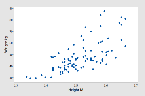
I hear you. To make this all a little more tangible, let’s take a look at an example of a correlation in action.
Here’s a scatter plot demonstrating the correlation (relationship) between weight and height. Intuitively, we’d expect there to be some relationship between these two variables, which is what we see in this scatter plot. In other words, the results tend to cluster together in a diagonal line from bottom left to top right.

As I mentioned, these are are just a handful of inferential techniques – there are many, many more. Importantly, each statistical method has its own assumptions and limitations.
For example, some methods only work with normally distributed (parametric) data, while other methods are designed specifically for non-parametric data. And that’s exactly why descriptive statistics are so important – they’re the first step to knowing which inferential techniques you can and can’t use.
To choose the right statistical methods, you need to think about two important factors:
Let’s take a closer look at each of these.
The first thing you need to consider is the type of data you’ve collected (or the type of data you will collect). By data types, I’m referring to the four levels of measurement – namely, nominal, ordinal, interval and ratio. If you’re not familiar with this lingo, check out the video below.
Why does this matter?
Well, because different statistical methods and techniques require different types of data. This is one of the “assumptions” I mentioned earlier – every method has its assumptions regarding the type of data.
For example, some techniques work with categorical data (for example, yes/no type questions, or gender or ethnicity), while others work with continuous numerical data (for example, age, weight or income) – and, of course, some work with multiple data types.
If you try to use a statistical method that doesn’t support the data type you have, your results will be largely meaningless. So, make sure that you have a clear understanding of what types of data you’ve collected (or will collect). Once you have this, you can then check which statistical methods would support your data types here.
If you haven’t collected your data yet, you can work in reverse and look at which statistical method would give you the most useful insights, and then design your data collection strategy to collect the correct data types.
Another important factor to consider is the shape of your data. Specifically, does it have a normal distribution (in other words, is it a bell-shaped curve, centred in the middle) or is it very skewed to the left or the right? Again, different statistical techniques work for different shapes of data – some are designed for symmetrical data while others are designed for skewed data.
This is another reminder of why descriptive statistics are so important – they tell you all about the shape of your data.
The next thing you need to consider is your specific research questions, as well as your hypotheses (if you have some). The nature of your research questions and research hypotheses will heavily influence which statistical methods and techniques you should use.
If you’re just interested in understanding the attributes of your sample (as opposed to the entire population), then descriptive statistics are probably all you need. For example, if you just want to assess the means (averages) and medians (centre points) of variables in a group of people.
On the other hand, if you aim to understand differences between groups or relationships between variables and to infer or predict outcomes in the population, then you’ll likely need both descriptive statistics and inferential statistics.
So, it’s really important to get very clear about your research aims and research questions, as well your hypotheses – before you start looking at which statistical techniques to use.
Never shoehorn a specific statistical technique into your research just because you like it or have some experience with it. Your choice of methods must align with all the factors we’ve covered here.
See how HAMNIC Solutions can help you...
You’re still with me? That’s impressive. We’ve covered a lot of ground here, so let’s recap on the key points:
Access to a wide variety of free tools, research templates, and guidelines can be obtained by visiting our website, which can be found here. We are always ready to provide you with comprehensive research guidance and project support in the event that you ever need assistance with writing your research project, review journal, article, or dissertation. At HAMNIC Solutions, our team of professionals and research experts is always ready to guide you through your research journey.